Economic analysis of natural hazard mitigation using the Quick Economic Analysis Tool

An effective way to reduce the impacts of natural hazards on communities is by mitigating the risks. However, mitigation requires time and resources, which are usually limited. To use resources effectively, planners and managers are best prepared when they know their options and which of these options provides the best value for money. When there is not enough information, or an analysis would take several months or years to complete, having access to quick economic analyses in weeks rather than months would be very useful. This paper describes a Quick Economic Analysis Tool, developed at the University of Western Australia, to conduct quick analyses. A case study is used of two prescribed burn annual rates and are compared with results of an in-depth analysis of the application of different prescribed burn annual rates over the long-term that took several years to complete. The results from the quick analysis, despite a few differences, were comparable to results from an in-depth analysis and provided enough information to determine the value for money that each prescribed burn annual rate generated. This study showed that the quick analysis tool would allow fire managers to identify options worthy of business cases and to capture the information needed to increase confidence in their decisions.

Introduction

Governments operate within limited budgets and they need to decide how to best allocate resources for effective mitigation activities of natural hazards. To be effective, natural hazard managers need to compare the costs and benefits of different options and identify the option that provides the best value for money. Ideally, this would be done through a comprehensive economic analysis that provides information on the net benefits of each option and the value for money expected from each dollar invested.

However, conducting this type of in-depth economic analysis can take a long time, from several months to several years (Florec et al. 2020; Penman, Bradstock & Price 2014). Even integrating new information, such as intangible (non-market) values, into an already completed analysis can take several months (Florec, Chalak & Hailu 2017). However, natural hazard managers may need economic information in a much shorter timeframe.

If there was a tool to help them get quick and accurate option(s) likely to generate the best returns on investment and the additional information needed, this could significantly speed up the decision-making process. It would also allow for decisions to be based on evidence and that trade-offs between different options are fully understood.

Such a tool has been developed for this purpose. The Quick Economic Analysis Tool (QEAT) is a spreadsheet-based model allowing a quick and rough overview of the value for money managers can expect from investing in various mitigation options. It includes tangible (market) and intangible (non-market) values that can be affected by natural hazards.

QEAT provides a way for planners and managers to conduct analyses in weeks (rather than months or years) to identify:

• the options that are worth developing business cases for
• the type of information needed to improve decisions and the confidence in them.

To test the tool, results obtained from a quick economic analysis of bushfire management in the south-west of Western Australia using QEAT were compared with the results of a comprehensive economic analysis already conducted. That analysis had taken four years to complete (Florec et al. 2020). This paper provides a summary of the arguments for and against using QEAT to evaluate mitigation options.

Methods

The Quick Economic Analysis Tool

QEAT is a spreadsheet that allows the user to insert relevant parameters and easily and quickly calculate benefit-cost ratios (BCRs) and net present values (NPVs). In this format, the value for money generated by the different options can be quickly compared. A sensitivity analysis can also be conducted to test the robustness of the results.

QEAT users must be clear about the counterfactual, that is, the baseline scenario to which the mitigation options are compared. For example, doing nothing, business as usual or other. This has the potential to increase transparency and reduce confusion sometimes associated with economic analyses of natural hazards. This occurs when practitioners are not clear about how the benefits are calculated.

The mathematical formulation of the model embedded in QEAT is:

• Compare option 1 to option x:
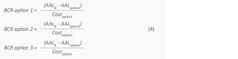
  • using net benefits:

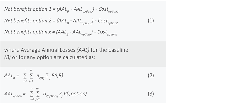
• and using BCRs:

In equation (2), η_i(B)j is the percentage of asset j destroyed by natural hazard event i for the baseline scenario (B), Z_j is the value (in dollars) of asset j, and P(i,B) is the probability of event i occurring under the baseline scenario (B).

In equation (3) the same parameters are used but for a scenario where one of the options is implemented. The implementation costs of each option (Cost_option) correspond to the annual costs of operations plus the initial fixed costs to set up the mitigation strategy.

Case study

In Western Australia, the south-west forests are managed by the Department of Biodiversity, Conservations and Attractions (DBCA). The South West region (see boundaries of the three forest regions in Figure 1) is approximately 1.88 million hectares and contains a mix of forests, coastal mallee shrublands and heathlands, agricultural land as well as residential areas. It has a Mediterranean-type climate with hot dry summers and mild wet winters. Bushfires of different severity occur every year in the region, particularly in the hotter months between October and May when the vegetation is dry and rainfall is minimal. The region has a long history of prescribed burning and complex fire management issues because of the combination of different land uses and tenures, where assets are intermingled with flammable vegetation.

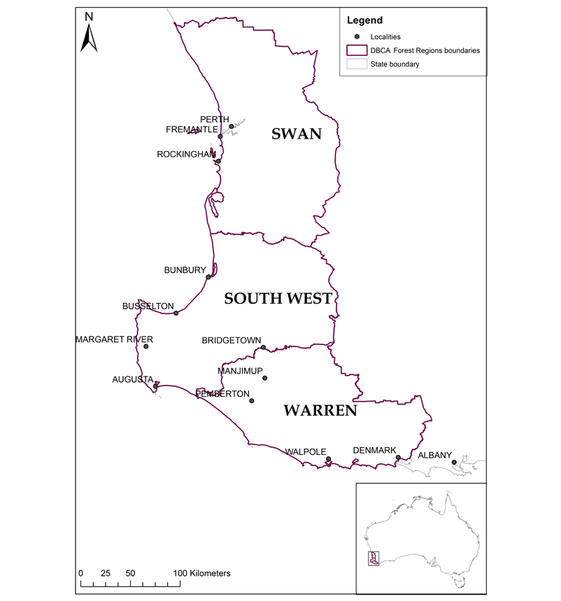
Figure 1: The south-western forest regions managed by the Department of Biodiversity, Conservation and Attractions.

Details of the analysis

Two prescribed burning annual rates were tested. These were prescribed burning five per cent and ten per cent of public land managed by the DBCA. These targets were selected as they were proposed in the literature as appropriate risk reduction targets for this region and for other regions in Australia. The ten per cent target corresponds to the area that would need to be treated annually in order to reach the areal extent necessary to protect communities, the environment and biodiversity (Burrows & McCaw 2013); while the five per cent target has been suggested for other regions in enquiries conducted after large and economically significant fire events (Teague, McLeod & Pascoe 2010). The counterfactual (to which mitigation strategies are compared) was doing nothing; that is, no prescribed burning. A 20-year timeframe was used for the analysis with a discount rate of seven per cent.

To populate the input parameters in QEAT, historical data for the south-west of Western Australia for the past 60 years was used. Most of the data is publicly available and included lives lost, properties destroyed, and, in some cases, area burnt. However, some of the data (hectares burnt and location of the area burnt) was obtained from DBCA. Although the level of prescribed burning applied in the wider south-west region has varied greatly over the last 80 years, several large wildfires have caused significant damages in the region:

• In 1961, 160 houses were destroyed and the town of Dwellingup was destroyed.
• In 1978, two lives were lost and six buildings destroyed; a narrow escape for four major towns.
• In 1997, two lives were lost, 21 injuries and 17 houses destroyed.
• In 2003, two lives were lost, more than two million hectares of forest were destroyed.
• In 2007, 16 houses destroyed in Dwellingup, three lives lost and a major highway closed for two weeks generating significant losses to some industries.
• In 2011, 34 houses were destroyed.
• In 2015, four lives were lost and a major highway was closed for several days, generating losses to the dairy industry.
• In 2016, two lives were lost, 181 properties were destroyed and the town of Yarloop was destroyed.

Table 1 shows the values used for each type of asset and their respective sources.

Table 1: Value of different assets.

Results

Table 2 shows the results obtained from QEAT. These results show that without mitigation, average annual losses could amount to $167 million. Most of the losses (61 per cent) stem from damage to buildings (residential, commercial and industrial buildings combined) followed by agricultural losses (about 25 per cent) and effects on human health (about nine per cent).

The results for the two prescribed burn scenarios (five and ten per cent of public land prescribed burnt) in Florec and colleagues (2020) are shown in Table 3. The categories of assets included there are different from those included in QEAT, where four categories were evaluated instead of five. The categories ‘urban’ and ’nature and conservation’ included in Florec and colleagues (2020) roughly correspond to the ‘buildings’ and ‘environment’ categories in this study, respectively. The category ‘infrastructure’ was not included in Florec and colleagues (2020). The main addition in this study was the improvement in information gained on non-market values for ‘human health’ and the ‘environment’. These were extracted from the Value Tool for Natural Hazards (Gibson et al. 2018), which is a database of non-market values relevant to natural hazards.

Table 2: Results with and without mitigation.

The results in Table 3 indicate that average annual losses without mitigation could amount to AU$232 million, which is about 21 per cent higher than the result from QEAT. The proportion of damage attributed to each category differs between QEAT and Florec and colleagues (2020). A much higher proportion of the losses in Table 3 stem from:

• damage to buildings of about 73 per cent of total damages
• environmental damages of about 14 per cent of losses, which is greater than what is indicated by QEAT
• agricultural damages of about six per cent, which is substantially less than what is indicated by QEAT.

Table 3: Results with and without mitigation from an existing published study.

Source: Florec et al. (2020)

Acknowledging these points of difference, there is a high degree of complementarity in the results, particularly from the perspective of the outcomes that would inform decision-making. Both models indicate that the implementation of the two prescribed burn scenarios (five per cent and ten per cent) in the case study area generated substantial benefits. Estimates from QEAT showed lower benefits from prescribed burning than those estimated by Florec and colleagues (2020). Therefore, the benefit-cost ratios from QEAT are also lower. Both prescribed burn scenarios generated good value for money in the case study area (i.e. BCRs were substantially higher than 1). Based on the BCRs, the five per cent scenario generated more value per dollar invested than the ten per cent scenario in both models. This suggests that prescribed burning has diminishing marginal returns; that is, after a certain point, every additional dollar invested in prescribed burning generates smaller and smaller benefits (which is consistent with previous studies (Mercer et al. 2007, Butry et al. 2010). However, based on NPVs, the ten per cent scenario provided better outcomes than the five per cent scenario (i.e. higher NPV), which makes it a more attractive strategy if the costs can be afforded.

Sensitivity analysis

Another important output of QEAT is the information it provides to planners and managers on the confidence they can have in the results and the information they need to increase that confidence. Results from a sensitivity analysis performed in QEAT for this purpose are shown in Table 4 and Table 5 for the five per cent and ten per cent prescribed burn scenarios, respectively.

Table 4: Sensitivity analysis prescribed burning five per cent.

^A Only the parameter indicated on each row is changed.
^B Damages are increased by a further 10%, 25% or 50%.
^C Damages are decreased by a further 10%, 25% or 50%.

Table 5: Sensitivity analysis prescribed burning ten per cent.

^A Only the parameter indicated on each row is changed.
^B Damages are increased by a further 10%, 25% or 50%.
^C Damages are decreased by a further 10%, 25% or 50%.

Although the results appear robust (i.e. the proportional change in the results is generally a lot smaller than the proportional change in the parameter), some parameters deserve attention. The asset categories in QEAT included the category ‘buildings’, which has a much stronger effect on the results than any other asset category. This was expected as the value of buildings is high compared to other assets and bushfires destroy buildings. The category ‘human health’ (life and injuries) also has high value, but loss of life and injuries caused by bushfires tend to be less common in the case study region, and therefore have less of an effect on the results. For fire managers, this means that having better information on how effective prescribed burning is for protecting buildings can provide better confidence levels in decisions and better allocation of funding for prescribed burning.

Another interesting parameter is the effectiveness of prescribed burning, or the capacity of the practice to reduce bushfire risk. For the five per cent prescribed burn, a change in the effectiveness of prescribed burning has a relatively high impact on the results; more so if the effectiveness is decreased. However, for the ten per cent strategy, a change in the effectiveness of prescribed burning has less impact on the results. For a fire manager, this means that if there are constraints on the area that can be burned and the area that can be treated is relatively small, treatments need to be targeted at protecting high-value assets. Thus, any changes in losses avoided have a high impact on the return on investment. But if larger areas can be burned, then the effectiveness of prescribed burning in reducing damage has a more moderate impact on the results and the confidence in the return on investment is higher.

Changes to prescribed burning costs have a very high impact on the results. Therefore, to increase the confidence in decisions for prescribed burns, it is important to have accurate data on costs of prescribed burning and to understand how these costs change for different prescribed burning activities.

Conclusion

The QEAT was used to conduct a quick analysis of two prescribed burning annual rates in the south-west of Western Australia. Results were compared with an in-depth analysis undertaken between 2012 and 2016. Despite some differences, the results from the QEAT were comparable to those of the in-depth analysis and provided sufficient information to determine the value for money that each annual rate generated. A sensitivity analysis conducted using QEAT demonstrated its capacity to show the types of additional information needed to increase the confidence in decisions made for prescribed burns. For the case study used, these were the data on the effectiveness of prescribed burning in reducing risk to buildings, data on the effects of prescribed burning when fuel loads are high in the region and data on prescribed burning costs.

Using QEAT, rapid and accurate information on the costs and benefits of different mitigation options can be obtained, thereby saving time and money to agencies that need this information. By understanding the confidence that can be attributed to different mitigation decisions and prioritising the additional data needed to increase the confidence in those decisions, the use of QEAT can improve outcomes for disaster risk reduction across Australia and possibly for other countries.

Glossary of economic terms

Benefit-cost ratio: Indicator used in benefit-cost analyses to measure the potential value for money that can be obtained from alternative investment options. It is calculated by dividing the benefits of an investment option by its costs. The BCR value (less than, equal to, or higher than 1) represents the benefits that can be expected for every dollar invested. For instance, a BCR value of 3:1 means that for every dollar invested, the option generates $3 in benefits.

Present value: The current value of a future sum of money or a future stream of cash flows for a given period and a specified rate of return. Because money has interest-earning potential, the value of a sum of money today (present value) is usually less than its future value.

Discount rate: The rate of return used to calculate present values. The discount rate selected for the analysis has an important impact on the results: the higher the discount rate, the lower the present value.

Net benefits: Calculated by subtracting the costs from the benefits.

Net present value: Calculated by subtracting the present value of costs from the present value of benefits.

Sensitivity analysis: A test of the robustness of the results of a study. A sensitivity analysis evaluates how the uncertainty in the results of a mathematical model can be attributed to different sources of uncertainty in its inputs.

Market values: Assets for which reconstruction costs or total value can be readily estimated in dollars, because these items are exchanged in markets and already have prices (i.e. items that are normally bought or sold).

Non-market values: Also referred to as social and environmental assets, non-market values concern those things that are not exchanged in markets (i.e. are not normally bought or sold) and therefore do not have a price (e.g. biodiversity, life).