The Excess Heat Factor as a metric for heat-related fatalities: defining heatwave risk categories
Thomas Loridan, Lucinda Coates, Daniel Argüeso, Sarah Perkins-Kirkpatrick, John McAneney
Peer-reviewed Article
Abstract
Article
Introduction
Heatwaves can have considerable economic and societal impacts (Nairn & Fawcett 2013) and are responsible for the largest number of deaths in Australia from natural disasters (Coates et al. 2014). However, there is no consensus about what constitutes a heatwave event (Perkins 2015) or even about the way one should go about quantifying heatwave intensity. Acknowledging this gap, Nairn and Fawcett (2015) designed a heatwave index to account for:
- the ability of local communities to adapt to its climate
- the dramatic effects that sharp temperature spikes can trigger through a lack of acclimatisation.
This metric, called the Excess Heat Factor (EHF), is an ideal method to homogenise the description of heatwave intensity from a hazard point of view. It also lends itself to the characterisation of various severity thresholds.
Using the 85th percentile of all positive EHF values from 1958-2011, Nairn and Fawcett (2015) define a severity classification scheme and label heatwave events as either low-intensity, severe or extreme. This approach is a natural step towards better risk communication. However, the implications of a high EHF are dependent on the risk being studied. For applications such as energy demand or infrastructure damage the threshold EHF values above which action needs to be taken will be significantly higher than when trying to accommodate, for instance, human discomfort and increased use of health services (Hatvani-Kovacs et al. 2015, Scalley et al. 2015). In this study the focus is on potential heat-related fatalities. The PerilAUS database (Coates et al. 1996) is used as an archive of deaths attributed to extreme heat conditions in Australia. From a ranking of the heatwave episodes associated to these deaths (in terms of EHF magnitude) a set of four heatwave severity categories is defined. These capture conditions that historically led to a greater number of deaths and should help communication about heat-related risks. Using Census population data to normalise the PerilAUS records, a fatality curve to link these categories to a potential death toll is used. This paper introduces a methodology to generate realistic, synthetic heatwave scenarios.
Excess Heat Factor
There have been many ways to define a heatwave event (Perkins 2015), however the EHF methodology introduced by Nairn and Fawcett (2013, 2015) is being adopted as the standard metric in Australia. It recognises the need to account for both minimum and maximum daily temperatures when assessing heatwave intensity, and explicitly separates the impact of short- and long-term temperature anomalies.
An excess heat index is computed to capture a-typical occurrences of high heat accumulation at a particular location in respect to that location’s long-term temperature average. For this purpose the daily mean temperature (TM) is calculated as the average of the daytime maximum and night-time minimum air temperatures over a three-day period compared to the 95th percentile of TM at the location of interest (TM95). Daily minimum and maximum temperature data for Australia are available from the Bureau of Meteorology from 1911 (Jones, Wang & Fawcett 2009). In this study the significant excess heat index (EHI) on day ‘i’ is defined as:
Equation 1:

A positive EHISIG indicates an unusually warm three-day period relative to the local climate statistics while all other days are assigned a value of zero.
An acclimatisation index (EHIACC) is brought into play to capture sudden rises in temperature in relation to the recent past. The index is computed in a similar fashion to Equation 1, this time comparing the three-day average to the past month (30-day) average:
Equation 2:
A positive value of EHIACC indicates a sharp temperature rise, to which the local population might not have time to acclimatise.
The EHF is obtained as a combination of EHISIG and EHIACC:
Equation 3:

The strengths of the EHF as a measure of heatwave occurrence and intensity are that it:
- is location dependent and explicitly acknowledges that populations in warmer climates are more resilient in the face of higher daily mean temperatures
- accounts for both short-term and climate-scale temperature anomalies.
The EHF can be used as an accumulated index characterising heat load over time. For that purpose, the daily EHF values are summed over a certain time period, such as the duration of the event. The resulting integrated value represents the heat load and accounts for both the event duration and its strength over time.
This raises the question: knowing the peak EHF intensity and heat load for a given event, can the severity of the risk to human life be anticipated?
Heat-related fatality risk potential
Defining heatwave categories
Having identified objective measures of heatwave severity, their potential link to heat-related fatalities are investigated from analysis of two data products. The PerilAUS archive (Coates et al. 1996) provides a list of 224 historical occurrences of heat-related deaths in Australia. The record includes the number of fatalities reported along with dates and locations. In addition, gridded records of daily minimum and maximum temperature available from the Australian Bureau of Meteorology since 1911 (5 km resolution Bureau of Meteorology dataset, Jones, Wang & Fawcett 2009) are used to compute EHF estimates for the 12-day period prior to the reported fatalities (a period of time long enough to cover most events durations). Both the maximum EHF over the period (EHFmax) and the 12-day accumulated heat load (EHFsum) are used to characterise the conditions that led to the fatalities. These two indices are computed from the average daily EHF value in the 10 km x 10 km boundary that contains the PerilAUS record location.
Figure 1 shows the 224 records, marked as dots and coloured in terms of the total number of fatalities reported on that day and in that location. The records are sorted by increasing order of the 12-day accumulated EHF (EHFsum, x-axis, Figure 1a) and 12-day maximum EHF (EHFmax, Figure 1b). The y-axis is the conditional exceedance frequency of that same quantity. From such a representation the relevance of the two metrics relating to the number of fatalities is clear: the most lethal records (warmer-coloured dots) are mainly to the right of the two figures (representing higher intensity heatwaves). It is also worth noting the cluster of points on the zero line as they represent fatalities for which the EHF definition would not have indicated the presence of a heatwave event.
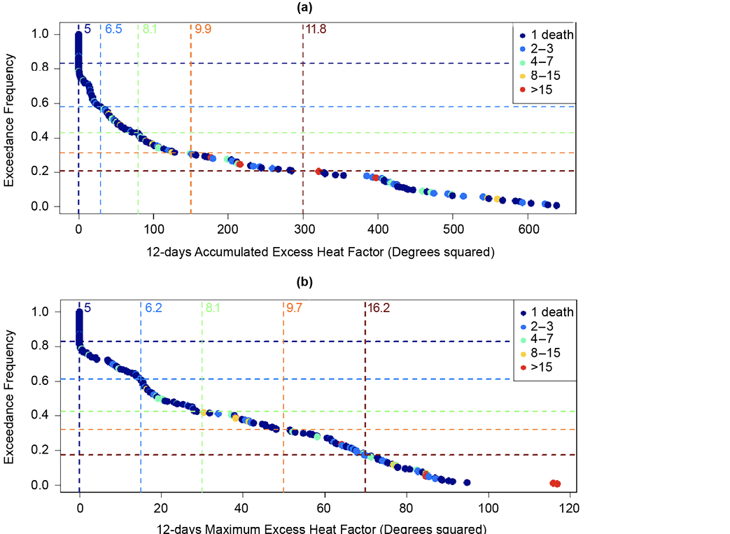
Figure 1: Conditional exceedance frequency as a function of (a) the accumulated EHF over the 12-day period prior to each reported fatality and (b) the maximum EHF over that period.
The vertical dashed lines represent various threshold values selected to group the data in different categories. The numerals next to them indicate the average death toll for all points situated to the right of that line. Note that one of the records reported over 300 fatalities (the February 2009 Victoria event, see Figure 4). The average for the last group of points is inflated as a consequence. Nonetheless the increasing trend in the mean number of deaths per occurrence suggests that both quantities are good indicators of heat-related fatalities (as the threshold values increase so does the number of fatalities per occurrence). One could therefore design a categorisation of events based on either one of these indicators for heatwave severity with regards to potential fatalities. Combining both metrics acknowledges that the most severe events will be characterised by both a large peak maximum (EHFmax) and a sustained period of high EHF (EHFsum). The combined classification scheme is provided in Table 1 along with key statistics for each category. It can be noted in Table 1 that the trend towards increasing numbers of fatalities per occurrence is greater than when the two indicators are treated separately. For each category, the equivalent (Nairn & Fawcett 2015) severity class is also reported for comparison based on the threshold EHF values for Melbourne and Adelaide.
Table 1: Criteria for the classification of heatwave events and statistics per category. Equivalent classes from the Nairn & Fawcett (2015) scheme are reported using the Melbourne and Adelaide threshold definitions.
| Category | EHFsum | EHFmax | Mean number of fatalities | Percentage of record covered | Equivalent NF15 class for Melbourne | Equivalent NF15 class for Adelaide |
|---|---|---|---|---|---|---|
|
CAT0 |
> 0 |
> 0 |
5 |
82.6 |
low-intensity |
low-intensity |
|
CAT1 |
> 30 |
> 15 |
6.7 |
55.4 |
low-intensity |
low-intensity |
|
CAT2 |
> 80 |
> 30 |
8.6 |
38.9 |
severe |
low-intensity |
|
CAT3 |
> 150 |
> 50 |
10.4 |
28.6 |
severe |
severe |
|
CAT4 |
> 300 |
> 70 |
18.5 |
12 |
extreme |
severe |
Application to the three worst events since 1900
To illustrate how the classification from Table 1 can be used to characterise specific events, three of the most lethal cases since 1900 in south-east Australia are analysed. For each, footprints of EHFmax and EHFsum values are first computed from the 5 km resolution Bureau of Meteorology dataset over the duration of the events. These are used to assign a category for each of the 5 km cells following the Table 1 scheme. Figures 2, 3 and 4 show the resulting category maps, along with records of fatalities (black dots, scaled in terms of the number of deaths). Unlike continuous maps of EHFmax or EHFsum values, these are direct representations of the risk gradient and can help illustrate the event to local populations. For comparison with the (Nairn & Fawcett 2015) severity categories, refer to their Figure 17 that covers the same event as in Figure 4. In both cases, most of south-east Australia is under the highest threat category.
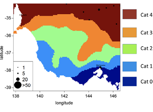
Figure 2: Map of Table 1 heatwave severity categories for the January 1939 event.
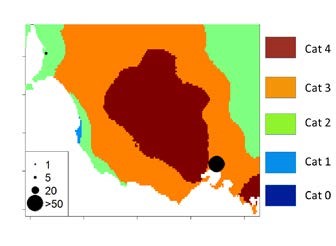
Figure 3: Map of Table 1 heatwave severity categories for the January 1959 event.
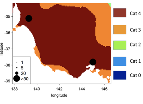
Figure 4: Map of Table 1 heatwave severity categories for the February 2009 event.
Heat-related fatality curve
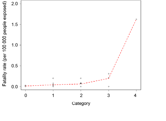
Figure 5: Rate of fatalities per 100 000 people (y-axis) as a function of the heatwave category they are exposed to (x-axis). Individual dots represent distinct events while the red dashed line is representative of all-events combined.
From knowledge of both peak and accumulated EHF estimates during a given event one can compute the associated category and apply the relationship from Figure 5 to project an expected number of fatalities.
Building a synthetic heatwave scenario
Hazard footprint
Using the methods described, a catalogue of historical events impacting south-east Australia since 1911 was assembled (see examples from Figures 2-4). To limit the number of events, only cases for which at least one 5 km grid cell in the domain has experienced a minimum of three consecutive days of positive EHF are considered. The 466 occurrences were characterised in a map of both the peak EHF during the duration of the event and its accumulated value. A detailed analysis of the key components of heatwave footprints in the region was undertaken with the aim of extrapolating the data from this catalogue beyond what has been experienced since 1911. For this purpose, the 466 peak and accumulated EHF footprints were decomposed using principal component analysis (PCA). The key idea at the core of PCA is that the footprints in the catalogue can be projected onto a family of vectors called empirical orthogonal functions (EOFs) that explain the variability observed since 1911. Mathematically the EOFs form a basis of orthogonal vectors and allow decomposition of the field of interest (i.e. either the peak EHF, EHFmax or its accumulated value EHFsum) using a set of event-specific coordinates zi(k). For instance, for the case of EHFmax, any event ‘k’ in the catalogue can be reconstructed starting from the mean footprint (MFP, see Figure 6) in the following way:
Equation 4:

The neofs is the total number of EOFs, which equals the number of grid points in the domain. With the EOFs ordered in terms of importance (based on the percentage of variance explained, see Figure 7) this decomposition enables analysis of the key patterns of variability (i.e. that explain more variance) among the 466 events in the catalogue. Furthermore, this reconstruction can easily be truncated to keep only the leading vectors. This provides a very practical way in which PCA can help generate synthetic events that are consistent with the observed historical variability.
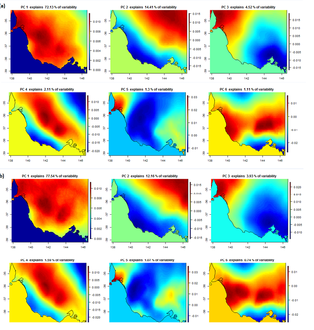
Figure 7: Top six Empirical Orthogonal Functions for the peak EHF magnitude and the accumulated EHF. Images provided by author.
For this study, the first six EOFs (i.e. set neofs to six in Equation 4) for both EHFsum and EHFmax were used. By assigning values to the associated EOF weights (zi in Equation 4) from analysis of their historical distributions, synthetic scenarios can be created to represent unseen cases that are consistent with the most typical observed patterns in the region. The leading six EOF fields used for this exercise are presented in Figure 7.To illustrate the outcome of this method a synthetic event (Figure 8) was designed to simultaneously impact the cities of Adelaide and Melbourne. It corresponds to synoptic situations where a high pressure system is preventing any relief from cooler maritime air masses.
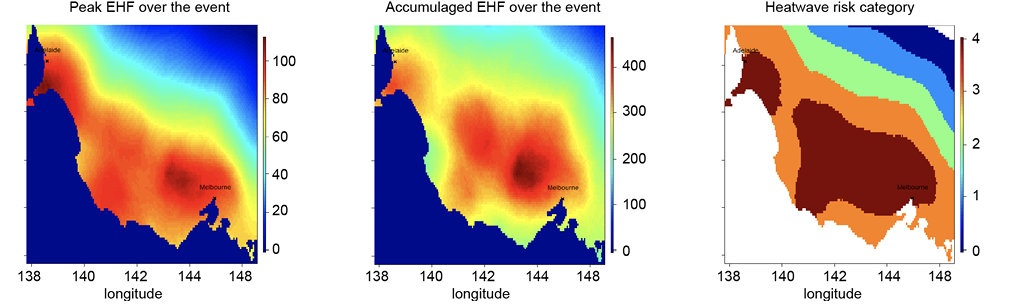
Figure 8: Synthetic event representing a coastal event affecting densely populated areas around Melbourne and Adelaide.
Projected fatalities
For the scenario shown in Figure 8, an estimate of the expected number of fatalities can be derived using the vulnerability curve from Figure 5. For this purpose, fatalities are simulated within each of the 5 km resolution cells that cover the domain from knowledge of the total population within a cell, and the heatwave category to which the population is exposed.
Using a binomial distribution, the number of deaths can be simulated to provide a picture of the geographical spread of fatalities. For this scenario, a total of 86 fatalities is expected in the region (see Figure 9) with both Adelaide and Melbourne sharing a significant proportion of the total. The large majority of cases are within the area under category 4 risk while some fatalities occur under the category 3 footprint.
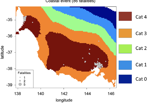
Figure 9: Simulated fatalities for the Figure 8 scenario (grey dots).
Conclusions
The EHF heatwave intensity framework was used in combination with an archive of heat-related fatalities in Australia to provide alternative indicators of heatwave severity. This led to the definition of four severity classes that may be helpful in characterising and communicating the potential of fatalities from heatwaves. These categories were depicted on a chart to show the risk of three important historical events affecting Victoria and South Australia.
The Bureau of Meteorology database of minimum and maximum temperature records dating from 1911 was used to assemble a catalogue of 466 historical heatwave events in south-east Australia. Each event was characterised by both peak and accumulated EHF estimates and PCA was applied to extract the key modes of variability. A synthetic scenario was constructed to represent a realistic event in metropolitan regions in Australia.
To quantify the effect of the scenario beyond the hazard threat, a vulnerability curve was defined to estimate the number of human fatalities that might be expected as a function of both the heatwave risk category and the population density. The method was applied to project the number and location of fatalities associated with the synthetic scenario.
It is worth mentioning that, as all estimates in this study are based on reported fatalities, and because of under-reporting and the likelihood of wrongly categorising deaths to other health-related issues rather than heat stress, fatality projections should be interpreted as lower-bound estimates. A more optimistic view would also acknowledge that communities and governments learn from past experience and improve their level of preparedness. In that sense, fatality rates from the last decade (Figure 5) might not accurately reflect the current level of awareness of the population and the ability of government services to cope with the threat. It is clear that to factor these two opposite views, some level of uncertainty around the estimates of Figure 5 needs to be modelled in future attempts to characterise heat-related fatality curves.
Study to date has focused on human fatalities attributed to heatwaves. A natural follow-up would be to look at non-lethal heat-related injuries. Following the framework introduced in this report, additional data, such as ambulance calls or hospitalisation records, would allow the development of complementary vulnerability curves and enable in-depth analysis of the effects of heatwaves on human health. Similarly, the fatality curve could be refined to capture the death-rate-by-age band or other characteristics of the degree of resilience of the local population. This would allow a better representation of the areas at risk.
Such considerations would be valuable input to assess the capability of emergency response services to cope. This framework might answer questions such as whether medical staff in local communities can handle the projected heat-related hospitalisations during extreme heat events.
| Acknowledgements
This research was funded by the Bushfire and Natural Hazards CRC through the ‘Using Realistic Disaster Scenario Analysis to Understand Natural Hazard Impacts and Emergency Management Requirements’ program. |
References
Coates L 1996, An overview of fatalities from some natural hazards. In: Heathcote RL, Cuttler C, Koetz J (Eds.) Proceedings NDR’96 Conference on Natural Disaster Reduction, Institution of Engineers Australia, 29 September–2 October 1996, Surfers Paradise, Queensland, pp. 49-54.
Coates L, Haynes K, O’Brien J, McAneney J & Dimer de Oliveira F 2014, Exploring 167 years of vulnerability: An examination of extreme heat events in Australia 1844-2010. Environ. Science and Policy 42, pp. 33-44.
Hatvani-Kovacs G, Belusko M, Pockett J & Boland J 2016, Can the Excess Heat Factor Indicate Heatwave-Related Morbidity? A Case Study in Adelaide, South Australia. EcoHealth (2016) 13: p. 100. doi:10.1007/s10393-015-1085-5
Jones DA, Wang W & Fawcett R 2009, High-quality spatial climate data-sets for Australia, Australian Meteorology Oceanographer Journal, 58, pp. 233-248.
Nairn J & Fawcett R 2013, Defining heatwaves: heatwaves defined as a heat impact event servicing all community and business sectors in Australia. CAWCR Technical report No 060. The Centre for Australian Weather and Climate Research.
Nairn J & Fawcett R 2015, The Excess Heat Factor: A metric for heatwave intensity and its use in classifying heatwave severity. International Journal of Environmental Research and Public Health, 12, pp. 227-253.
Perkins S 2015, A review on the scientific understanding of heatwaves – Their measurement, driving mechanisms, and changes at the global scale. Atmospheric Research, pp. 164-165, pp. 242-267.
Scalley BB, Spicer T, Jian L, Xiao J, Nairn J, Robertson A & Weeramanthri T 2015, Responding to heatwave intensity: Excess Heat Factor is a superior predictor of health service utilisation and a trigger for heatwave plans. Australia New Zealand Journal of Public Health 2015 December, vol. 39. no. 6, pp. 582-587. doi: 10.1111/1753-6405.12421
About the authors
Dr Thomas Loridan is a lead scientist at Risk Frontiers specialising in atmospheric hazard modelling with a particular emphasis on tropical cyclones. He holds a PhD from King’s College London where he studied models of the urban boundary layer. In the past five years his work has led to the development of various techniques to simulate the variability in severe winds observed from cyclones across the world’s most active basins. More recently his research has also focused on developing risk metrics for heatwaves in Australia.
Lucinda Coates is a Catastrophe Risk Scientist at Risk Frontiers. Areas of interest include risk reduction and climate change adaptation assessment among the community, trends in Australian natural hazard fatalities, vulnerability verses resilience and evaluations of risk perception and risk communication. Lucinda has worked on a number of projects for the Australian emergency management sector and government and private organisations.
Dr Daniel Argüeso is a Postdoctoral Research Fellow at University of Hawai’i at Manoa. His research includes improvement of tropical cyclone forecast using lightning. He has a background in atmospheric physics and climate modelling. He has investigated features of present and future climate in different regions using regional climate models. He also works on urban climate, tropical convection, sea-breeze, heatwaves and extra-tropical cyclones
Dr Sarah Perkins-Kirkpatrick is a climate scientist studying heatwaves. She has a PhD from UNSW Australia and is currently an Australian Research Council DECRA fellow at the same institution. Sarah has undertaken work investigating the measurement of heatwaves, their observed changes, future projections from climate models, and the human contribution behind these changes. Sarah received a NSW Young Tall Poppy award in 2013 for science communication, was shortlisted for a 2014 Eureka science prize as part of the UNSW Extremes Team and was recently named one of UNSW’s 20 rising stars who will change the world.
Professor John McAneney is Managing Director of Risk Frontiers and has expertise in probabilistic modelling, quantitative risk assessment and cost benefit and real options analyses. He has over 130-refereed publications on various aspects of weather risk, boundary layer physics and natural peril risks.